1. Basic Facts about the Gamma Function
The Gamma function is defined by the improper integral
The integral is absolutely convergent for since
and is convergent. The preceding
inequality is valid, in fact, for all . But for
the integrand becomes infinitely large as approaches through
positive values. Nonetheless, the limit
exists for since
for , and, therefore, the limiting value of the preceding integral
is no larger than that of
Hence, is defined by the
first formula above for all values .
If one integrates by parts the integral
writing
with and , one obtains the functional
equation
Obviously, , and, therefore,
,
,
, …, and, finally,
for each integer .
Thus, the gamma function provides a way of giving a meaning to the
“factorial” of any positive real number.
Another reason for interest in the gamma function is its relation
to integrals that arise in the study of probability. The graph of the
function defined by
is the famous “bell-shaped curve” of probability theory. It can be
shown that the anti-derivatives of are not expressible in
terms of elementary functions. On the other hand,
is, by the fundamental theorem of calculus, an anti-derivative of
, and information about its values is useful.
One finds that
by observing that
and that upon making the substitution in the latter
integral, one obtains .
To have some idea of the size of , it will be useful
to consider the qualitative nature of the graph of .
For that one wants to know the derivative of .
By definition is an integral (a definite integral with
respect to the dummy variable ) of a function of and
. Intuition suggests that one ought to be able to find the
derivative of by taking the integral (with respect to )
of the derivative with respect to of the integrand.
Unfortunately, there are examples where this fails to be correct; on
the other hand, it is correct in most situations where one is inclined
to do it. The methods required to justify “differentiation under the
integral sign” will be regarded as slightly beyond the scope of this
course. A similar stance will be adopted also for differentiation of
the sum of a convergent infinite series.
Since
one finds
and, differentiating again,
One observes that in the integrals for both and the second
derivative the integrand is always positive. Consequently,
one has and for all . This
means that the derivative of is a strictly increasing
function; one would like to know where it becomes positive.
If one differentiates the functional equation
one finds
where
and, consequently,
Since the harmonic series diverges, its partial sum in the foregoing
line approaches as . Inasmuch as
, it is clear that approaches
as since is steadily increasing
and its integer values approach .
Because ,
it follows that cannot be negative everywhere in the interval
, and, therefore, since is increasing,
must be always positive for . As a result, must be
increasing for , and, since , one sees
that approaches as .
It is also the case that approaches as
. To see the convergence one observes that the
integral from
to defining is greater than the integral from
to of the same integrand. Since for
, one has
It then follows from the mean value theorem combined with the fact that
always increases that approaches
as .
Hence, there is a unique number for which ,
and decreases steadily from to the minimum value
as varies from to and then increases to
as varies from to . Since
, the number must lie in the interval
from to and the minimum value must be less than .
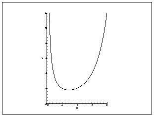
Figure 1: Graph of the Gamma Function |
Thus, the graph of (see Figure 1) is concave upward
and lies entirely in the first quadrant of the plane. It has the
-axis as a vertical asymptote. It falls steadily for
to a postive minimum value . For the graph
rises rapidly.
2. Product Formulas
It will be recalled, as one may show using l'Hôpital's Rule,
that
From the original formula for , using an interchange of limits
that in a more careful exposition would receive further comment, one has
where is defined by
The substitution in which is replaced by leads to
the formula
This integral for is amenable to integration by parts.
One finds thereby:
For the smallest value of , , integration by parts yields:
Iterating times, one obtains:
Thus, one arrives at the formula
This last formula is not exactly in the form of an infinite product
But a simple trick enables one to maneuver it into such an infinite
product. One writes as a “collapsing product”:
or
and, taking the th power, one has
Since
one may replace the factor by in the last expression above
for to obtain
or
The convergence of this infinite product for when
is a consequence, through the various maneuvers performed, of the
convergence of the original improper integral defining for
.
It is now possible to represent as the sum of an infinite
series by taking the logarithm of the infinite product formula. But first
it must be noted that
Hence, the logarithm of each term in the preceding infinite product is
defined when .
Taking the logarithm of the infinite product one finds:
where
It is, in fact, almost true that this series converges absolutely for
all real values of . The only problem with non-positive
values of lies in the fact that is meaningful only for
, and, therefore, is meaningful only for
. For fixed , if one excludes the finite set of terms
for which , then the remaining “tail” of
the series is meaningful and is absolutely convergent.
To see this one applies the “ratio
comparison test” which says that an infinite series converges absolutely
if the ratio of the absolute value of its general term to the general
term of a convergent positive series exists and is finite. For this
one may take as the “test series”, the series
Now as approaches , approaches ,
and so
Hence, the limit of is , and the series
is absolutely convergent for all real . The absolute
convergence of this series foreshadows the possibility of defining
for all real values of other than non-positive integers.
This may be done, for example, by using the functional equation
or
to define for and from there
to , etc.
Taking the derivative of the series for term-by-term
– once again a step that would receive justification in a more careful
treatment – and recalling the previous notation for the
derivative of , one obtains
where denotes Euler's constant
When one has
and since
this series collapses and, therefore, is easily seen to sum to .
Hence,
Since , one finds:
and
These course notes were prepared while consulting standard references
in the subject, which included those that follow.